Current Research (by Area)
My Research Statement:
1. Stochastic Algorithm for Nonsmooth Nonconvex-Nonconcave Minmax Problem
Background: The nonconvex-nonconcave minmax problem is an important issue arising in operations management and machine learning theory. For example, many operational objectives are formulated in a minmax setting $\min_{x}\max_{y}f(x,y)$, where $x$ and $y$ are real-valued vectors and $f$ is neither (necessarily) convex in $x$ nor (necessarily) concave in $y$. Without solid assumptions on $f$, this problem might be intractable. However, it might be even trickier with complicated constraints for $(x,y)$. There are also a few classical applications for nonconvex-nonconcave minmax problem in machine learning theory, such as the training of generative adversarial networks (GANs) or robust neural-nets. The typical Wasserstein GAN (WGAN) objective is defined as the minimization of the Wasserstein distance between the discriminator $D_y$ of the true distribution $b$ and that of the one learnt by the generator $G_x$ as follows,
\[\min\limits_x \max\limits_{y} \mathbb{E}_{\beta\sim b} [D_y(\beta)] - \mathbb{E}_{\alpha\sim a}[D_y(G_x(\alpha))],\]where $G_x$ might not be convex in $x$ for all $y$ and/or $D_y$ not be concave in $y$ for all $x$ in this saddle point problem. There may also be constraints on $x$ and $y$, which results in a complicated constrained nonconvex-nonconcave minmax problem.
Research Direction: To identify the solutions of this type problem, we have 3 research directions.
VI/MI: The minmax optimization problem can be cast as a special case of variational inequality problems (VIPs) or monotone inclusion problems (MIPs). Therefore, by identifying stochastic algorithms that achieve the optimal convergence rate in generalized MIPs or VIPs, we are able to attain the saddle points or stationary points under certain convergence rate for a family of structured nonconvex-nonconcave minmax optimization problems.
Weak Assumption: Another line of our work is to ensure the convergence under the weaker assumptions of convexity-concavity, such as the two-sided Polyak-Łojasiewicz condition or $\rho$-weakly convex-concave assumption.
Normal Map (Main Direction): Especially for nonsmooth case, we introduce normal mapping to offer a normal map-based method to resolve the biasedness of some stochastic proximal methods like prox-SGDA and to measure the convergence of these methods by converting the expectation of the natural residual into a normal mapped one.
Normal Map-based Method: We study the following nonsmooth nonconvex-nonconcave minmax problem
\[\min\limits_x \max\limits_{y}\ \ \psi(x,y) = \mathbb{E}_{\delta\sim \Delta}[f(x,y;\delta)]+\varphi(x)-h(y),\]where $f: \mathbb{R}^{2n} \rightarrow \mathbb{R}$ is Lipschitz smooth and not (necessarily) convex-concave in $z=(x,y)$, while $\varphi: \mathbb{R}^n \rightarrow \mathbb{\bar{R}}$ and $h: \mathbb{R}^n \rightarrow \mathbb{\bar{R}}$ are convex in $x$ and $y$, respectively. The proximity operator of $\varphi$ at $x$ and $h$ at $y$ can be expressed as,
\[\begin{align} \textrm{prox}_{\alpha_{k}\varphi}(x) &:= \textrm{arg}\min_{p\in \mathbb{R}^n} \{\varphi(p)+ \frac{1}{2\alpha_k}||x-p||^2 \},\\ \textrm{prox}_{\alpha_{k}h}(y) &:= \textrm{arg}\max_{q\in \mathbb{R}^n} \{-h(q)- \frac{1}{2\alpha_k}||y-q||^2 \}. \end{align}\]Given the above proximities are nonlinear operators, the unbiasedness of the random gradient in stochastic proximal methods would be lost. Consider the proximal Stochastic Gradient Descent Ascent (prox-SGDA) as an example,
\[\begin{align} \mathbb{E}_{k}[x^{k+1}]&=\mathbb{E}_{k}[\textrm{prox}_{\alpha_{k}\varphi}(x^{k}-\alpha_{k}g_{x}^{k})] \color{DarkGoldenRod}{\neq \textrm{prox}_{\alpha_{k}\varphi}(x^{k}-\alpha_{k}\nabla_{x} f(x^{k},y^{k}))},\\ \mathbb{E}_{k}[y^{k+1}]&=\mathbb{E}_{k}[\textrm{prox}_{\alpha_{k}h}(y^{k}+\alpha_{k}g_{y}^{k})] \color{DarkGoldenRod}{\neq \textrm{prox}_{\alpha_{k}h}(y^{k}+\alpha_{k}\nabla_{y} f(x^{k},y^{k}))}, \end{align}\]which cannot recover prox-GDA due to the nonlinear proximity operator. To address the biasedness of the stochastic estimator in prox-SGDA, we thus seperate proximity operators from the update process and introduce the normal map to capture the gradient and subgradient of $\psi$. Let $x := \textrm{prox}_{\lambda \varphi} (u)$ and $y:=\textrm{prox}_{\lambda h} (v)$, then the normal maps are given as,
\[\begin{align} F_{nor}^{\lambda}(u)&: = \nabla_x f(x,y)+\frac{1}{\lambda}(u-x) \in \nabla_x f(x,y)+ \partial \varphi(x),\\ F_{nor}^{\lambda}(v)&: = \nabla_y f(x,y)-\frac{1}{\lambda}(v-y) \in \nabla_y f(x,y)- \partial h(y). \end{align}\]When $F_{nor}^{\lambda}(u) = F_{nor}^{\lambda}(v) = 0$, $z = (x,y)$ is the stationary point of $\psi$. Based on $F_{nor}^{\lambda}(u)$ and $F_{nor}^{\lambda}(v)$, we then define the normal maps as new descent and ascent directions for $u$ and $v$, with additional proximal updating to $x$ and $y$. Thus, we provide the following Normal Map-based SGDA Algorithm, which can be seen as a special subgradient method,
\[\textrm{Loop:} \left\{\begin{matrix} \begin{aligned} &g^k \approx \nabla f(x^k,y^k) \ \ \ \ \ \ \ \ \ \ \ \ \ \ \ \ \color{DarkGoldenRod}{\textrm{by some sampling scheme}} \\ &u^{k+1} = u^k-\alpha_k (g_x^k + \frac{1}{\lambda}(u^k-x^k)) \color{DarkGoldenRod}{\approx u^k - \alpha_k F_{nor}^{\lambda}(u^k)}\\ &v^{k+1} = v^k+\alpha_k (g_y^k - \frac{1}{\lambda}(v^k-y^k)) \color{DarkGoldenRod}{\approx v^k + \alpha_k F_{nor}^{\lambda}(v^k)}\\ &x^{k+1} = \textrm{prox}_{\lambda \varphi} (u^{k+1})\\ &y^{k+1} = \textrm{prox}_{\lambda h} (v^{k+1}) \end{aligned} \end{matrix}\right. \tag{9}\]where the updates are unbiased, i.e.,
\[\begin{align} \mathbb{E}_{k}[u^{k+1}] &= u^k-\alpha_k (\nabla_{x}f(x^k,y^k) + \frac{1}{\lambda}(u^k-x^k)), \tag{10}\\ \mathbb{E}_{k}[v^{k+1}] &= v^k+\alpha_k (\nabla_{y}f(x^k,y^k) - \frac{1}{\lambda}(v^k-y^k)). \tag{11} \end{align}\]Given the proposed Normal Map-based SGDA Algorithm, a convergent and optimistic version can also be formulated by replacing $g^k$ in $(9)$ with $g^{k+1}$ approximated by $(1+\frac{\alpha}{\beta})g^{k}+\frac{\alpha}{\beta}g^{k-1}$ (or a Normal Map-based Extragradient Algorithm by replacing $g^k$ with $g^{k+\frac{1}{2}}$ approximated by $g^{k-\frac{1}{2}}-g^{k}+g^{k-1}$). With diminishing step sizes $\color{DarkGoldenRod}{\alpha_{k} = O(1/k^{\gamma})}$, we obtain strong convergence $\lim \limits_{k\to \infty}x^{k} = x^{*} \in \textrm{crit}(\psi)$ almost surely in nonconvex-nonconcave case, and we have,
\[||x^{k}-x^{*}||= \left\{\begin{matrix} \begin{aligned} &O(1/\sqrt{k}), \ \ \ \ \ \ \ \ \ \ \ \ \ \ \ \ \ \ \ \ \ \ \ \ \ \ \ \ \ \ \ \ \ \ \ \ \textrm{if}\ \theta \in [0,1/2],\\ &O(1/k^{p}), p\in (0,1/2), \ \ \ \ \ \ \ \ \ \ \ \ \ \ \ \ \textrm{if}\ \theta \in (1/2,1),\\ \end{aligned} \end{matrix}\right. \tag{12}\]where $\theta \in [0,1)$ is the KL exponent. Similar strong convergence results can also be obtained and proved in the Normal Map-based Extragradient Algorithm in accordance with the Supermartingale Convergence Theorem and KL inequality, whereby we show that $\{x^{k}\}_k$ is convergent.
(Bonus) Useful Lemma from Normal Map: In comparison to the natural residual $F_{nat}^{\lambda}(x)$, the normal map $F_{nor}^{\lambda}(z)$ can be employed as a tighter merit (gap) function in the convergence analysis for nonconvex cases, which also helps to convert the expectation of natural residual $\mathbb{E}[F_{nat}^{\lambda}(x)]$ into a better-solved equation when analyzing stochastic algorithms.
\[\begin{aligned} ||F_{nat}^{\lambda}(x)|| &= ||\textrm{prox}_{\lambda \varphi} (z) - \textrm{prox}_{\lambda \varphi}(x-\lambda \nabla f(x))||,\\ &\leq ||z-x+\lambda \nabla f(x)||, \ \ \ \ \color{DarkGoldenRod}{\textrm{(Non-expansiveness)}}\\ & = \lambda ||F_{nor}^{\lambda}(z)||, \end{aligned} \tag{13}\]where the natural residual $F_{nat}^{\lambda}(x)\leq \epsilon$ can be ensured under $ \lambda F_{nor}^{\lambda}(z)\leq \epsilon$ after $k$ iterations, when $x=\textrm{prox}_{\lambda \varphi} (z)$.
Our Contribution: The main contributions of this research project can be summarized as follows.
First stochastic algorithm to resolve the biasedness of stochastic methods in nonsmooth or constrained case.
First strong convergence result for stochastic proximal-type algorithm in nonconvex-nonconcave case.
The rate $O(1/\sqrt{k})$ matches that of OGDA in strongly convex setting. Additionally, the rate $O(1/\sqrt{k})$ is tight.
Current Progress: The paper is quite long and technical, so we still need time to check some technical details including proofs and conduct more experimemts. Articles are expected to submit to some journals or conferences in 2024.
- Yilin Gu, Andre Milzarek (2024). Normal Map-Based Proximal Extragradient Methods for Nonsmooth Nonconvex-Nonconcave Minmax Problem.
- Yilin Gu, Andre Milzarek (2024). Convergence of A Revised Foward-Backward-Foward Method for Nonsmooth Nonconvex-Nonconcave Minmax Problem.
The following presentation slides introduce the main ideas and some technical details of this paper.
Normal Map Slides: [slides].
2. Adaptive Multiple Vector Quantization Classification (Master Thesis)
Background: Learning Vector Quantization (LVQ) is a family of algorithms for statistical pattern classification, which aims at learning a prototype for each class to represent class regions. Despite the simpleness and efficiency, the prototypes of LVQ-type algorithms work well in hyper-spherical classes. However, current LVQ with its variants often suffer from poor performance when training nonconvex pattern classes, which obviously cannot be represented by a single prototype thus hard to capture the nonconvex pattern in a specific class. Also, because of the non-convexity of these models, LVQ-type algorithms encounter difficulties in finding global optimal solutions and further suffering bad convergence.

The goal of this research is to modify Learning Vector Quantization (LVQ) algorithm well known in prototype classification and provide our new algorithm Adaptive Multiple Vector Quantization (AMVQ) to better capture the nonconvex and sparse pattern of classes with improved interpretation, convergence, and simplicity, particularly for production-related data.
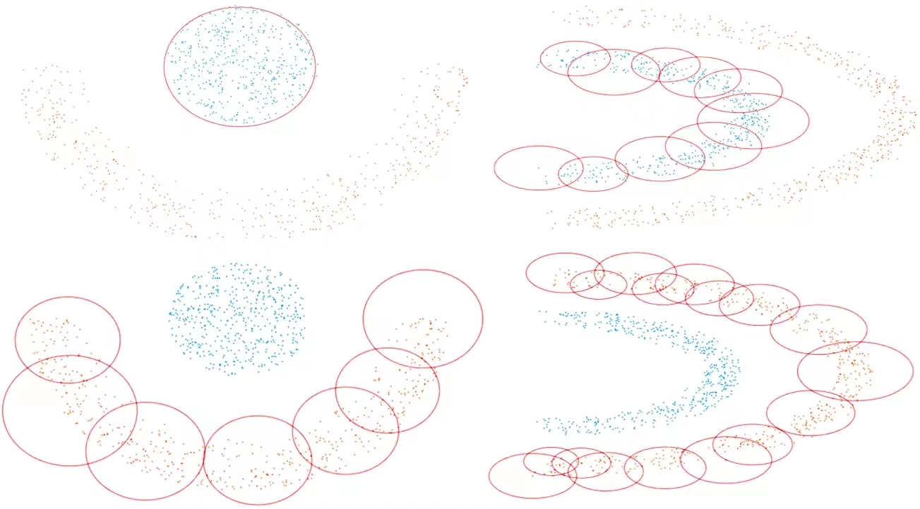
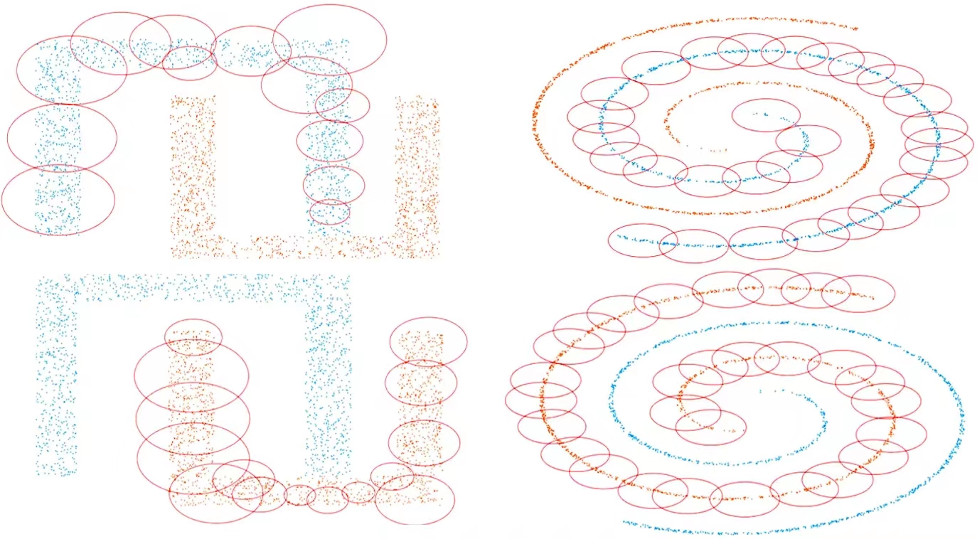
Adaptive Multiple Vector Quantization: In order to capture the nonconvex and sparse pattern of classes, we provide a multiple-prototype adaptive vector quantization model that sample points in each class can be fully covered by prototypes’ decision domains. Nevertheless, having too many prototypes will increase the complexity of the model and reduce robustness throughout the training and prediction process. Therefore, our task is to employ the fewest number of prototypes necessary to cover all of the sample points in each class inside the prototypes’ decision domains. Then, we write our task into an optimization problem,
\[\min_{A^k}\ f(A^k) = \sum_{i=1}^{m_k} ||x_i^k-A^k||_{\textrm{hub}}-m_{k}\cdot r_{A^k}, \tag{1}\]where $A^k \in \mathbb{R}^n$ is the prototype for class $k$, while $x_i^k \in \mathbb{R}^n$ and $m_k \in \mathbb{R}$ are the sample points and the number of sample points for class $k$, respectively. The $r_{A^k}\in \mathbb{R}$ is the decision region radius of the prototype $A^k$, which can be measured as the huber distance between prototype $A^k$ and its closest sample points in other classes $-k$,
\[r_{A^k} = \min\{||x_1^{-k}-A^k||_{\textrm{hub}},...,||x_{m_{-k}}^{-k}-A^k||_{\textrm{hub}}\}. \tag{2}\]Due to the non-convexity of $(2)$, we linearize all the huber distances in $(2)$ to concavify $(2)$,
\[||x_i^{-k}-A^k||_{\textrm{hub}} \approx \left\{\begin{matrix} \begin{aligned} &\overbrace{\frac{1}{2\delta}||x_i^{-k}-A^{k,p}||^{2}_{2}+\frac{1}{\delta}(x_i^{-k}-A^{k,p})^\top A^{k,p}}^{\color{DarkGoldenRod}{b_i}} \overbrace{ - \frac{1}{\delta}(x_i^{-k}-A^{k,p})^\top}^{\color{DarkGoldenRod}{w_i}} A^{k}, \ \ \ \ \ \ \ \ \ \ \ \textrm{if}\ ||x_i^{-k}-A^{k}||_{2}\leq \delta,\\ &\overbrace{||x_i^{-k}-A^{k,p}||_{2}-\frac{(A^{k,p}-x_i^{-k})^\top A^{k,p}}{||x_i^{-k}-A^{k,p}||_{2}}-\frac{1}{2}\delta}^{\color{DarkGoldenRod}{b_i}}+\overbrace{(\frac{A^{k,p}-x_i^{-k}}{||x_i^{-k}-A^{k,p}||_{2}})^\top}^{\color{DarkGoldenRod}{w_i}} A^k, \ \ \ \textrm{if}\ ||x_i^{-k}-A^{k}||_{2}> \delta,\\ \end{aligned} \end{matrix}\right. \tag{3}\]where $A^{k,p}\in \mathbb{R}^n$ is the value of $A^{k}$ in the $p^{\textrm{th}}$ iteration. With the linearized huber distance in $(3)$, the concavified $(2)$ enables us to rewrite $(1)$ as the minimization of a convex function,
\[\min_{A^k}\ f(A^k) = \overbrace{\sum_{i=1}^{m_k} ||x_i^k-A^k||_{\textrm{hub}}}^{\color{DarkGoldenRod}{g(A^k)}}\overbrace{-m_{k}\cdot \min\{\color{DarkGoldenRod}{w_{1}}^{\top}A^{k}+\color{DarkGoldenRod}{b_{1}},...,\color{DarkGoldenRod}{w_{m_{-k}}}^{\top}A^{k}+\color{DarkGoldenRod}{b_{m_{-k}}}\}}^{\color{DarkGoldenRod}{h(A^k)}}, \tag{4}\]where $g: \mathbb{R}^{n} \rightarrow \mathbb{R}$ is (convex) smooth but $h: \mathbb{R}^{n} \rightarrow \mathbb{R}$ is (convex) nonsmooth in $A^k$. Therefore, we apply the proximal method to solve the nonsmooth problem $(4)$ and the proximity operator of $h$ at $A^k$ can be written as,
\[\textrm{prox}_{\lambda h}(A^k) := \textrm{arg}\min_{v\in \mathbb{R}^n} \{h(v)+ \frac{1}{2\lambda}||A^k-v||^2 \}= w^{-1}\cdot \max\{-m_{k}b-t^{\star}\textbf{1}, m_{k}w^{\top}A^k\}, \tag{5}\]with variables $w \in \mathbb{R}^{m_{-k}}$, $b \in \mathbb{R}^{m_{-k}}$, and $t^{\star}\in \mathbb{R}$ satisfies $\sum_{i=1}^{m_{-k}}\frac{1}{\lambda m_{k}^2 w_{i}^{\top}w_{i}}(-m_{k}b_{i}-m_{k}w_{i}^{\top}A^{k}-t^{\star})_{+}=1$, where $t^{\star}$ can be solved by bisection method with the interval $[\min_i(-m_{k}b_{i}-m_{k}w_{i}^{\top}A^{k}-\frac{1}{m_{-k}}),\max_i(-m_{k}b_{i}-m_{k}w_{i}^{\top}A^{k})]$. Thus, $(4)$ can be solved with a closed-form solution and we apply the accelerated proximal gradient method to identify prototypes,
\[\textrm{Loop:} \left\{\begin{matrix} \begin{aligned} &y^p = (1-\theta_p)A^{k,p-1}+\theta_{p}u^{p-1}\\ &A^{k,p} = \textrm{prox}_{h\lambda}(y^p-\lambda_p \nabla g(y^p))\\ &u^{p} = A^{k,p-1}+\frac{1}{\theta_p}(A^{k,p}-A^{k,p-1})\\ &\theta_p = \frac{2}{p+1} \end{aligned} \end{matrix}\right. \tag{6}\]When we obtain the $j^{\textrm{th}}$ optimal prototype $A_j^k$ for class $k$ throughout $(6)$, we eliminiate all the sample points covered by the decision domain of $A_j^k$ and use the remaining sample points to find the next optimal prototype $A_{j+1}^k$, until all the points (or a specific rate of the points) in class $k$ have been covered. Simultaneously, we employ the following trust region-type strategy to force our iterations to stop with the fewest possible prototypes,
\[\begin{align} &\frac{\Gamma_{p-1}-\Gamma_{p}}{\Delta r_p} \leq \eta_1 \cdot \min\{\frac{\Gamma_{p-2}-\Gamma_{p-1}}{\Delta r_{p-1}},...,\frac{\Gamma_{0}-\Gamma_{1}}{\Delta r_1}\},\ \eta_1 \in (0,1), \tag{7}\\ &\frac{\Gamma_{p-1}-\Gamma_{p}}{\Delta r_p} \geq \eta_2 \cdot \max\{\frac{\Gamma_{p-2}-\Gamma_{p-1}}{\Delta r_{p-1}},...,\frac{\Gamma_{0}-\Gamma_{1}}{\Delta r_1}\},\ \eta_2 \in (1,+\infty), \tag{8} \end{align}\]where $\Gamma_p = \sum_{i=1}^{m_k}\textrm{sign}({\left\Vert x_i^k-A^{k,p}\right \Vert -r_p})$ for the $p^{\textrm{th}}$ iteration (specifically we rule $\Gamma_0 = m_k$) and $\Delta r_p = \left\Vert r_p-r_{p-1} \right\Vert$. When the iteration of $A^{k}$ reaches the point where $(7)$ is satisfied, it suggests that we should stop our iteration because we won’t get many marginal covered points even if we keep raising the radius of the prototype’s decision region significantly. As a result, it stops us from increasing the radius too much and making the model non-robust. While $(8)$ is fulfilled, it indicates that the sample points covered by the prototype shift from a sparse region to a condense one, which allows us to discriminate between the sparsity of samples with prototypes. With backtracking step sizes $\lambda_{\min} = \min \{1,\beta/L\}$, we obtain the optimal linear convergence $O(1/k^2)$ rate to find the global optimal solution for prototype $A^k$ and some fascinating experiment findings on capturing nonconvex and irregular pattern in classification problem shown as follows,


Given the above training process obtaining all the prototypes from each class, we predict the class $\kappa$ of any new data point $x_{\textrm{new}}$ by identifying the prototype $A^k$ that matches the smallest distance between $x_{\textrm{new}}$ and the decision boundary of $A^k$,
\[\kappa(x_{\textrm{new}}) := \textrm{arg} \min\limits_{A^k} ||x_{\textrm{new}}-A^k||-r(A^k), \tag{9}\]from which we can classify the class of $x_{\textrm{new}}$ as that of $A^{k\star}$ from $(9)$ in this supervised classification problem.
Our Contribution: The main contributions of this research project can be summarized as follows.
First adaptive multiple prototype model that obtains the fewest number of prototypes without prior knowledge.
First prototype-based model that captures prototype with a global optimal closed-form solution.
In contrast to the fixed radius model, AMVQ identifies prototypes in a radius-descent order, which automatically generates the importances and shows the decision region of prototypes for better model interpretation.
Achieves the optimal $O(1/k^2)$ convergence rate and the least $O(1/\sqrt{\epsilon})$ iteration complexity in identifying prototypes.
Current Progress: The master thesis is almost finished and expected to submit (after necessary revisions). Here are the Matlab codes, proposal and some drafts of this paper.
AMVQ codes: [codes].
AMVQ Abstract: [abstract].
- Yilin Gu, Andre Milzarek, Yichen Yu, Xin Jin, and Ruiyun Xu (2024). Stepwise Prototype Optimization: Adaptive Multiple Vector Quantization Classification.
